Table of Contents
I was very pleased to wake up the other day to find that some code I wrote for the ordered logistic distribution had been accepted into TensorFlow Probability (TFP)! However when writing this post I found that my code wasn't quite right (so my testing was bad) and I've tried to rectify that in this PR which includes the code I am using in this post.
The ordered logistic distribution is one of those annoying ones which people tend to call lots of different things and also write down differently too. The implementation I used in TFP follows Stan and PyMC3 and is currently documented here.
I've decided to show an example of all this with some soccer data, in fact the same data I used in a previous post when I diagnosed a problem with the model underestimating the draw probability. I wonder if it will be the case again when we directly consider modelling the (clipped) score difference as an ordered outcome?
I'll also implement the model in TFP and Stan and see how they compare.
For a detailed explanation on the prior used on the cutpoints and general ordinal model goodness, see this case study by Michael Betancourt.
1 Setup
Until the next TFP release (0.10.0 I think) the ordered logistic distribution will be available in the nightly TFP release, which is tested against the TensorFlow nightly release:
import tensorflow as tf
import tensorflow_probability as tfp

print(f"tf: {tf.__version__}")
print(f"tfp: {tfp.__version__}")
tf: 2.2.0-dev20200212
tfp: 0.10.0-dev20200214
2 Data
import pandas as pd
import numpy as np

data_list = []
for x in range(10, 19):
    season = f"{x}{x+1}"
    url = f"http://www.football-data.co.uk/mmz4281/{season}/E0.csv"
    data_list.append(pd.read_csv(url))

soccer_data = (
    pd.concat(data_list, axis=0)
    .rename(
        columns={
            "HomeTeam": "home_team_name",
            "AwayTeam": "away_team_name",
            "FTHG": "home_goals",
            "FTAG": "away_goals",
        }
    )
    .filter(regex="^home_|^away_")
    .dropna()
    .astype({"home_goals": np.int32, "away_goals": np.int32})
    .assign(
        clipped_score_difference=lambda x: np.clip(
            x["home_goals"] - x["away_goals"], -3, 3
        )
    )
)

team_names = np.unique(
    pd.concat([soccer_data["home_team_name"], soccer_data["away_team_name"]])
)


def team_code(team_name):
    def fn(df):
        codes = pd.Categorical(df[team_name], categories=team_names).codes
        return codes.astype(np.int32)

    return fn


soccer_data = soccer_data.assign(
    home_team=team_code("home_team_name"), away_team=team_code("away_team_name"),
)

print(soccer_data.head())
  home_team_name away_team_name  home_goals  away_goals  \
0    Aston Villa       West Ham           3           0
1      Blackburn        Everton           1           0
2         Bolton         Fulham           0           0
3        Chelsea      West Brom           6           0
4     Sunderland     Birmingham           2           2

   clipped_score_difference  home_team  away_team
0                         3          1         32
1                         1          3         12
2                         0          5         13
3                         3         10         31
4                         0         27          2
3 TFP
num_outcomes = 7
num_teams = len(team_names)
home_team = soccer_data["home_team"].to_numpy()
away_team = soccer_data["away_team"].to_numpy()
clipped_score_difference = soccer_data["clipped_score_difference"].to_numpy()

tfb = tfp.bijectors
tfd = tfp.distributions

Root = tfd.JointDistributionCoroutine.Root


def logit(x):
    return -tf.math.log(tf.math.reciprocal(x) - 1.0)


def make_cutpoints(simplex):
    return logit(tf.math.cumsum(simplex[..., tf.newaxis, :-1], axis=-1))


def model():
    cutpoints_simplex = yield Root(tfd.Dirichlet([2.0, 4.0, 6.0, 8.0, 6.0, 4.0, 2.0]))
    team_scale = yield Root(tfd.HalfNormal(1.0))
    unit_team_strength = yield Root(tfd.MultivariateNormalDiag(loc=tf.zeros(num_teams)))

    team_strength = team_scale[..., tf.newaxis] * unit_team_strength
    home_strength = tf.gather(team_strength, home_team, axis=-1)
    away_strength = tf.gather(team_strength, away_team, axis=-1)

    clipped_score_difference = yield tfd.Independent(
        tfd.OrderedLogistic(
            cutpoints=make_cutpoints(cutpoints_simplex),
            loc=home_strength - away_strength,
        ),
        reinterpreted_batch_ndims=1,
    )


joint_dist = tfd.JointDistributionCoroutine(model)
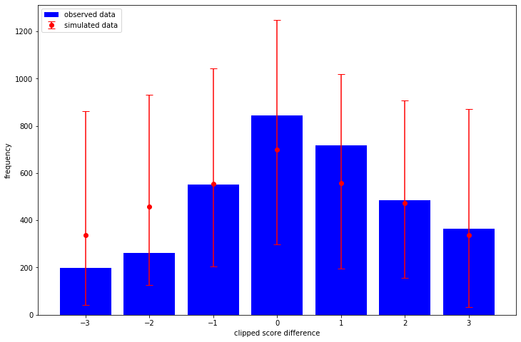
What I like about TFP over stan is that it is automatic to sample from the prior (i.e. before we condition on any observed outcomes) and in this case it is obvious what the effect of our priors are. That is, how informative and realistic they are. Here I sample 1,000 datasets and consider the resulting clipped score differences:
import matplotlib.pyplot as plt

plt.rcParams["figure.figsize"] = (12, 8)

_, _, _, prior_predictive_samples = joint_dist.sample(1_000)

sampled_score_difference_counts = [
    np.bincount(sample, minlength=7) for sample in prior_predictive_samples
]
observed_score_difference_counts = np.bincount(clipped_score_difference + 3)

sampled_mean = np.mean(sampled_score_difference_counts, axis=0)
sampled_quantiles = np.quantile(
    sampled_score_difference_counts, q=[0.025, 0.975], axis=0
)

low_error = sampled_mean - sampled_quantiles[0]
high_error = sampled_quantiles[1] - sampled_mean

plt.bar(
    x=np.arange(-3, 4),
    height=observed_score_difference_counts,
    label="observed data",
    color="blue",
)

plt.errorbar(
    x=np.arange(-3, 4),
    y=sampled_mean,
    yerr=[low_error, high_error],
    fmt="o",
    label="simulated data",
    color="red",
    capsize=5,
)

plt.legend(loc="upper left")
plt.xlabel("clipped score difference")
plt.ylabel("frequency")
The way we have written the model is quite interpretable - so we could spend some time thinking about what priors we should choose. That's not what I'm exploring in this post however - I want to see how my posterior looks!
I'm not quite sure how to decide how many chains/samples to take with TFP on the GPU right now, adding extra chains is usually cheap though so I'm running twice as many chains (and half the number of results) compared to the stan code below. I also just totally guessed the step size, I should probably check what step sizes the warmup finds to get a feel for the typical values of them.
import time as tm

num_chains = 10
num_burnin_steps = 1_000
num_results = 500


def target_log_prob_fn(*state):
    return joint_dist.log_prob(list(state) + [clipped_score_difference + 3])


def trace_fn(states, pkr):
    return (
        pkr.inner_results.inner_results.target_log_prob,
        pkr.inner_results.inner_results.leapfrogs_taken,
        pkr.inner_results.inner_results.has_divergence,
        pkr.inner_results.inner_results.energy,
        pkr.inner_results.inner_results.log_accept_ratio,
    )


def step_size_setter_fn(pkr, new_step_size):
    return pkr._replace(
        inner_results=pkr.inner_results._replace(step_size=new_step_size)
    )


def step_size_getter_fn(pkr):
    return pkr.inner_results.step_size


def log_accept_prob_getter_fn(pkr):
    return pkr.inner_results.log_accept_ratio


initial_state = list(joint_dist.sample(num_chains)[:-1])
initial_step_size = [0.25] * len(initial_state)

nuts = tfp.mcmc.NoUTurnSampler(target_log_prob_fn, step_size=initial_step_size)

transformed_nuts = tfp.mcmc.TransformedTransitionKernel(
    inner_kernel=nuts, bijector=[tfb.SoftmaxCentered(), tfb.Softplus(), tfb.Identity()],
)

adaptive_transformed_nuts = tfp.mcmc.DualAveragingStepSizeAdaptation(
    inner_kernel=transformed_nuts,
    num_adaptation_steps=int(0.8 * num_burnin_steps),
    target_accept_prob=0.8,
    step_size_setter_fn=step_size_setter_fn,
    step_size_getter_fn=step_size_getter_fn,
    log_accept_prob_getter_fn=log_accept_prob_getter_fn,
)


@tf.function(autograph=False, experimental_compile=False)
def run_mcmc():
    return tfp.mcmc.sample_chain(
        num_results=num_results,
        current_state=initial_state,
        num_burnin_steps=num_burnin_steps,
        kernel=adaptive_transformed_nuts,
        trace_fn=trace_fn,
    )
start_tfp = tm.time()
samples, sample_stats = run_mcmc()
end_tfp = tm.time()

print(f"TFP took {end_tfp - start_tfp:.2f} seconds")
TFP took 349.02 seconds
Was unfortunate that I couldn't get experimental_compile=True to work, which in some
examples gives a massive speed boost. It gives an error about the Gamma sampler not
being supported, which is called in the Dirichlet sampler.
As per usual I use arviz to explore the results:
import arviz as az
import numpy as np


sample_names = ["cutpoints_simplex", "team_scale", "unit_team_strength"]
summary_vars = ["mean", "sd", "hpd_3%", "hpd_97%", "ess_bulk", "r_hat"]

az_samples = {
    name: np.swapaxes(sample, 0, 1) for name, sample in zip(sample_names, samples)
}

sample_stats_names = [
    "lp",
    "tree_size",
    "diverging",
    "energy",
    "mean_tree_accept",
]

az_sample_stats = {
    name: np.swapaxes(stat, 0, 1)
    for name, stat in zip(sample_stats_names, sample_stats)
}

tfp_fit = az.from_dict(
    az_samples,
    sample_stats=az_sample_stats,
    coords={"teams": team_names},
    dims={"unit_team_strength": ["teams"]},
)

print(az.summary(tfp_fit).filter(items=summary_vars))
                         mean     sd  hpd_3%  hpd_97%  ess_bulk  r_hat
cutpoints_simplex[0]    0.042  0.003   0.037    0.048    4994.0   1.00
cutpoints_simplex[1]    0.064  0.004   0.057    0.072    4757.0   1.00
cutpoints_simplex[2]    0.162  0.006   0.150    0.173    5277.0   1.00
cutpoints_simplex[3]    0.283  0.008   0.268    0.299    4781.0   1.00
cutpoints_simplex[4]    0.233  0.008   0.218    0.246    5265.0   1.00
cutpoints_simplex[5]    0.134  0.006   0.123    0.145    5321.0   1.00
cutpoints_simplex[6]    0.081  0.004   0.073    0.089    9180.0   1.00
team_scale              0.616  0.081   0.473    0.771     886.0   1.01
unit_team_strength[0]   1.726  0.310   1.175    2.335     985.0   1.00
unit_team_strength[1]  -0.663  0.262  -1.161   -0.173    1151.0   1.01
unit_team_strength[2]  -0.341  0.445  -1.174    0.487    1761.0   1.00
unit_team_strength[3]  -0.562  0.355  -1.201    0.125    1764.0   1.01
unit_team_strength[4]  -0.568  0.470  -1.447    0.320    2019.0   1.00
unit_team_strength[5]  -0.541  0.367  -1.237    0.132    1927.0   1.00
unit_team_strength[6]  -0.320  0.288  -0.874    0.218    1483.0   1.01
unit_team_strength[7]  -0.479  0.357  -1.152    0.194    1607.0   1.00
unit_team_strength[8]  -0.274  0.279  -0.814    0.233    1509.0   1.00
unit_team_strength[9]  -1.252  0.384  -1.997   -0.572    1383.0   1.01
unit_team_strength[10]  1.782  0.314   1.158    2.338     936.0   1.00
unit_team_strength[11] -0.025  0.252  -0.473    0.485    1230.0   1.00
unit_team_strength[12]  0.729  0.246   0.272    1.188    1002.0   1.00
unit_team_strength[13] -0.565  0.280  -1.082   -0.035    1306.0   1.00
unit_team_strength[14] -1.375  0.382  -2.064   -0.616    1391.0   1.00
unit_team_strength[15] -0.724  0.324  -1.325   -0.102    1659.0   1.00
unit_team_strength[16]  0.521  0.274   0.013    1.040    1323.0   1.00
unit_team_strength[17]  1.665  0.308   1.108    2.276     986.0   1.01
unit_team_strength[18]  2.524  0.382   1.836    3.265     905.0   1.01
unit_team_strength[19]  1.779  0.315   1.205    2.369     942.0   1.00
unit_team_strength[20] -0.616  0.448  -1.433    0.245    1766.0   1.01
unit_team_strength[21] -0.143  0.240  -0.593    0.308    1160.0   1.01
unit_team_strength[22] -0.551  0.291  -1.133   -0.043    1427.0   1.01
unit_team_strength[23] -0.759  0.317  -1.329   -0.137    1557.0   1.00
unit_team_strength[24] -0.868  0.443  -1.717   -0.048    1559.0   1.00
unit_team_strength[25]  0.293  0.251  -0.176    0.756    1190.0   1.00
unit_team_strength[26] -0.100  0.232  -0.544    0.329    1062.0   1.01
unit_team_strength[27] -0.367  0.251  -0.825    0.104    1206.0   1.01
unit_team_strength[28] -0.026  0.243  -0.474    0.436    1150.0   1.00
unit_team_strength[29]  1.482  0.291   0.921    2.018     967.0   1.00
unit_team_strength[30] -0.205  0.282  -0.740    0.333    1444.0   1.00
unit_team_strength[31] -0.191  0.232  -0.605    0.271    1080.0   1.00
unit_team_strength[32] -0.013  0.241  -0.479    0.439    1199.0   1.00
unit_team_strength[33] -0.563  0.309  -1.165   -0.013    1530.0   1.01
unit_team_strength[34] -0.538  0.328  -1.169    0.056    1612.0   1.00
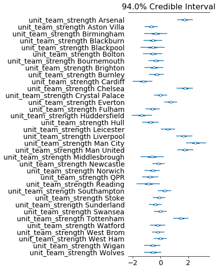
az.plot_forest(tfp_fit, var_names="unit_team_strength", combined=True)
4 Stan
Note that there is a bug in the current version of pystan with the ordered logistic distribution so we need to edit some C++ code as per this PR.
data {
    int<lower = 1> n;
    int<lower = 2> num_teams;
    int<lower = 2> num_outcomes;
    int<lower = 1, upper = num_teams> home_team[n];
    int<lower = 1, upper = num_teams> away_team[n];
    int<lower = 1, upper = num_outcomes> clipped_score_difference[n];
}

parameters {
    simplex[num_outcomes] cutpoints_simplex;
    vector[num_teams] unit_team_strength;
    real<lower = 0.0> team_scale;
}

model {
    vector[num_outcomes - 1] cutpoints = logit(
        cumulative_sum(cutpoints_simplex[1:(num_outcomes - 1)]));
    vector[num_teams] team_strength = team_scale * unit_team_strength;
    vector[n] location = team_strength[home_team] - team_strength[away_team];

    cutpoints_simplex ~ dirichlet([2.0, 4.0, 6.0, 8.0, 6.0, 4.0, 2.0]');
    unit_team_strength ~ std_normal();
    team_scale ~ std_normal();

    clipped_score_difference ~ ordered_logistic(location, cutpoints);
}
import pystan
import arviz as az

go_faster_flags = ["-O3", "-march=native", "-ffast-math"]

stan_model = pystan.StanModel(
    file=stan_file, model_name="ordered_model", extra_compile_args=go_faster_flags
)

stan_data = {
    "n": len(soccer_data),
    "num_teams": len(team_names),
    "num_outcomes": 7,
    "home_team": soccer_data["home_team"] + 1,
    "away_team": soccer_data["away_team"] + 1,
    "clipped_score_difference": soccer_data["clipped_score_difference"] + 4,
}

start_stan = tm.time()
stan_fit = az.from_pystan(
    stan_model.sampling(data=stan_data, chains=5),
    coords={"team": team_names},
    dims={"unit_team_strength": ["team_names"]},
)
end_stan = tm.time()

print(f"stan took {end_stan - start_stan:.2f} seconds")
stan took 22.13 seconds
print(az.summary(stan_fit).filter(items=summary_vars))
                         mean     sd  hpd_3%  hpd_97%  ess_bulk  r_hat
cutpoints_simplex[0]    0.042  0.003   0.037    0.048    9153.0    1.0
cutpoints_simplex[1]    0.064  0.004   0.057    0.071    8836.0    1.0
cutpoints_simplex[2]    0.162  0.007   0.150    0.174    8737.0    1.0
cutpoints_simplex[3]    0.283  0.008   0.268    0.299    8388.0    1.0
cutpoints_simplex[4]    0.233  0.008   0.219    0.248    9650.0    1.0
cutpoints_simplex[5]    0.134  0.006   0.123    0.145   10152.0    1.0
cutpoints_simplex[6]    0.081  0.005   0.073    0.090    8664.0    1.0
unit_team_strength[0]   1.725  0.307   1.133    2.282    1015.0    1.0
unit_team_strength[1]  -0.663  0.265  -1.164   -0.156    1107.0    1.0
unit_team_strength[2]  -0.356  0.448  -1.170    0.499    3462.0    1.0
unit_team_strength[3]  -0.564  0.365  -1.253    0.121    2398.0    1.0
unit_team_strength[4]  -0.586  0.469  -1.468    0.293    3941.0    1.0
unit_team_strength[5]  -0.549  0.374  -1.244    0.154    2431.0    1.0
unit_team_strength[6]  -0.326  0.291  -0.901    0.182    1396.0    1.0
unit_team_strength[7]  -0.477  0.350  -1.153    0.143    1982.0    1.0
unit_team_strength[8]  -0.272  0.294  -0.842    0.258    1401.0    1.0
unit_team_strength[9]  -1.234  0.384  -1.994   -0.550    2082.0    1.0
unit_team_strength[10]  1.781  0.310   1.194    2.353    1058.0    1.0
unit_team_strength[11] -0.019  0.261  -0.506    0.483    1102.0    1.0
unit_team_strength[12]  0.732  0.243   0.301    1.203     998.0    1.0
unit_team_strength[13] -0.565  0.279  -1.072   -0.032    1235.0    1.0
unit_team_strength[14] -1.378  0.386  -2.129   -0.655    1751.0    1.0
unit_team_strength[15] -0.722  0.328  -1.338   -0.111    1454.0    1.0
unit_team_strength[16]  0.521  0.273   0.039    1.055    1291.0    1.0
unit_team_strength[17]  1.664  0.301   1.088    2.215    1024.0    1.0
unit_team_strength[18]  2.525  0.373   1.814    3.207    1031.0    1.0
unit_team_strength[19]  1.779  0.308   1.202    2.356    1048.0    1.0
unit_team_strength[20] -0.609  0.458  -1.441    0.295    3138.0    1.0
unit_team_strength[21] -0.143  0.242  -0.615    0.295    1001.0    1.0
unit_team_strength[22] -0.550  0.293  -1.100   -0.009    1303.0    1.0
unit_team_strength[23] -0.756  0.322  -1.400   -0.184    1558.0    1.0
unit_team_strength[24] -0.859  0.449  -1.689   -0.023    3073.0    1.0
unit_team_strength[25]  0.295  0.243  -0.171    0.742    1089.0    1.0
unit_team_strength[26] -0.096  0.243  -0.525    0.387    1070.0    1.0
unit_team_strength[27] -0.366  0.252  -0.824    0.109    1067.0    1.0
unit_team_strength[28] -0.026  0.244  -0.483    0.427    1043.0    1.0
unit_team_strength[29]  1.481  0.287   0.961    2.034     995.0    1.0
unit_team_strength[30] -0.202  0.280  -0.734    0.311    1353.0    1.0
unit_team_strength[31] -0.188  0.242  -0.645    0.250     980.0    1.0
unit_team_strength[32] -0.011  0.238  -0.459    0.431     951.0    1.0
unit_team_strength[33] -0.570  0.315  -1.138    0.030    1676.0    1.0
unit_team_strength[34] -0.530  0.317  -1.089    0.091    1488.0    1.0
team_scale              0.615  0.080   0.480    0.773    1012.0    1.0
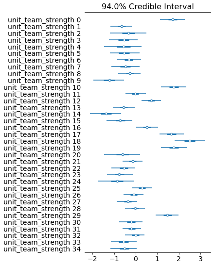
az.plot_forest(stan_fit, var_names="unit_team_strength", combined=True)
5 Posterior predictive check
Not sure how to implemenent this without copy-pasting some of the model code, would be awesome if there is a more automatic way, like when we take prior samples. Much of this code is the same as for the prior check, execpt I had to pin the sampling operation to the CPU as my (cheap) GPU would run out of memory otherwise.
cutpoints_simplex, team_scale, unit_team_strength = samples

team_strength = team_scale[..., tf.newaxis] * unit_team_strength
home_strength = tf.gather(team_strength, home_team, axis=-1)
away_strength = tf.gather(team_strength, away_team, axis=-1)

posterior_predictive_dist = tfd.OrderedLogistic(
    cutpoints=make_cutpoints(cutpoints_simplex),
    loc=home_strength - away_strength,
)

with tf.device("/CPU:0"):
    posterior_predictive_samples = posterior_predictive_dist.sample()

sampled_score_difference_counts = [
    np.bincount(sample, minlength=7)
    for sample in tf.reshape(posterior_predictive_samples, [-1, len(soccer_data)])
]

sampled_mean = np.mean(sampled_score_difference_counts, axis=0)
sampled_quantiles = np.quantile(
    sampled_score_difference_counts, q=[0.025, 0.975], axis=0
)

low_error = sampled_mean - sampled_quantiles[0]
high_error = sampled_quantiles[1] - sampled_mean

plt.bar(
    x=np.arange(-3, 4),
    height=observed_score_difference_counts,
    label="observed data",
    color="blue",
)

plt.errorbar(
    x=np.arange(-3, 4),
    y=sampled_mean,
    yerr=[low_error, high_error],
    fmt="o",
    label="simulated data",
    color="red",
    capsize=5,
)

plt.legend(loc="upper left")
plt.xlabel("clipped score difference")
plt.ylabel("frequency")
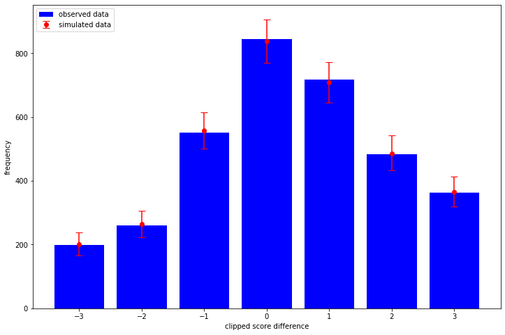
So no obvious problems with the model in this test!
6 Conclusion
I've skipped over a bunch of details in the code here, but hopefully this shows how one
might start using the new OrderedLogistic class in TFP and serves as another example
of how to run NUTS in TFP with a comparison with Stan.